Specifications for illumination systems for biomedical imaging and industrial metrology generally converge on spectral, spatial and temporal light output characteristics. This article describes some of the ways in which solid-state Light Engines consisting of arrays of solid-state light sources, a mix of LEDs, light pipes and lasers, allow for the customization of specifications to meet application-specific lighting requirements.

A solid-state Light Engine is a centrally controlled array of solid-state light sources whose outputs merge into a common optical train (Figure 1). The source outputs can be activated in parallel to generate white light (Figure 2), or sequentially (Figures 3, 4) when discrete wavelengths are needed. The sources themselves may be engineered from one solid-state lighting technology, namely LEDs, light pipes, or diode lasers, or some combination of source technologies, as dictated by the brightness, angular distribution and irradiance requirements of the end-user application. According to this definition, the spectral distribution of the Light Engine output can be assembled additively. This is in contrast to traditional broad spectrum illuminators like arc discharge and incandescent lamps which generate physically invariant spectral distributions which can only be adjusted by selective blocking and attenuation. From an engineering point of view, a second major advantage of solid-state light sources is that their output can be exquisitely controlled with respect to both intensity (Figures 2, 4) and time (Figures 4, 5). Consequently, the inter-unit variance of spectral output is low (Figure 2), resulting in consistent data quality from one imaging system to another.

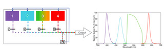
Figure 1. Conceptual depiction of a solid-state light engine and its spectral output. The outputs of four solid-state light sources are merged into a common optical train and coupled to a microscope
or image scanner via a light guide. In practice, the number of sources can be anywhere from 2–21, depending on application requirements. The light sources may be LEDs, light pipes, or diode lasers or a mixture of all three. Their outputs may be filtered (F) for spectral refinement. A fraction of the light output is split off and directed to a reference photodiode (rPD) to provide control feedback.

In most biomedical imaging applications continuous illumination is not required and, in some cases may even be contraindicated. Typically, illumination is synchronized with camera exposures. Two aspects are critical; first, inter-source switching speed and second, inter-pulse reproducibility. Inter-source switching in less than 1 millisecond (Figure 4) reduces the time required to acquire multicolor image z-stacks or slide scans relative to a white-light illuminator coupled to a mechanical filter wheel (~50 ms switching). Pulse-to-pulse integral invariance (Figure 5) is a critical determinant of time-lapse image sequence fidelity. The integral of each pulse quantifies the illumination applied to each exposure in the time-lapse sequence. Lower pulse-to-pulse illumination variance translates to increased sensitivity to the dynamic behavior of the specimen, manifested as changes from one image frame to the next.

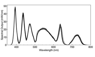
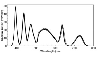
Figure 2. Overlaid spectral output curves for 28 individual SOLA V-nIR Light Engines (Lumencor, Inc., Beaverton OR). The total light output from the Light Engine is quantified by the area enclosed by the spectral output curve. Mean output power for all 28 Light Engines was determined to be 4558 mW, with a standard deviation (n= 28) of 91 mW, equating to a 2% coefficient of variance (CV).

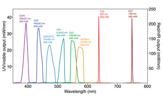
Figure 3. Spectral output of a SPECTRA Light Engine (Lumencor, Inc., Beaverton OR) incorporating LEDs, luminescent light pipes and lasers. Wavelength specifications for the LEDs and light pipes represent the center wavelength (CWL)/full-width half maximum (FWHM) in nanometers (nm) of the internal filters used to refine the source output. Power values in milliwatts (mW) are measured at the distal end of the light guide used to couple the light engine to a microscope or optical scanner. Integration of the three different types of solid-state light sources provides uniform power output across the visible spectrum and into near-infrared wavelengths.

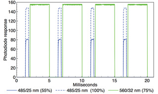
Figure 4. Oscilloscope recording of alternating 485 nm (0.5 ms width) and 560 nm (3 ms width) output pulses generated by TTL triggering of an AURA Light Engine (Lumencor, Inc., Beaverton, OR). Two superimposed oscilloscope traces are shown in which the 485 nm intensity is adjusted from 100% to 55% via RS232 serial commands while the 560 nm intensity remains constant. Temporal separation of the 485 nm and 560 nm pulses is ~0.25 ms.

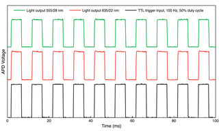
Figure 5. Trains of 5 ms light output pulses from a 5-source AURA Light Engine (Lumencor, Inc., Beaverton, OR) detected by an analog photodiode (APD). The plots show sequences of 10 pulses, representative of 150 successive pulses recorded in each data acquisition. The integral light output was calculated for each pulse in the 150-pulse train. For the 555/28 nm output, the coefficient of variance (CV) across 150 pulses was 0.23% for the 555/28 nm pulse train and 0.20% for 635/22 nm. Similar CV values (0.15–0.25%) were obtained for the other three source channels.

Apart from spectral bandwidth (Figure 3), the key difference between solid-state LEDs, light pipes and lasers is in the angular distribution of their light output; LEDs and lasers demonstrate the largest differences as quantified in Table 1. For widefield microscopy applications, LED sources configured for Köhler illumination [1] generate uniform illumination with irradiance in the range 1-100 mW/mm² [2]. However, single-molecule localization microscopy (SMLM) requires much higher irradiance, on the order of 10⁴ mW/mm² at the sample plane, provided by a laser Light Engine (CELESTA Light Engine, Lumencor, Inc., Beaverton, OR) coupled to a critical epilluminator installed in the microscope (Figure 6). The use of critical illumination [1] is dictated by the fact that Köhler illumination is optically inefficient because it does not encompass the entire surface of the light source or the full angular distribution of the emitted light. Critical illumination, in which the light source is imaged directly onto the sample plane, is more efficient but also more sensitive to any spatial non-uniformity in the light source output. The critical epilluminator acts to homogenize any spatial non-uniformity to produce a high-irradiance illumination field matched to the dimensions (~200 mm²) of typical sCMOS camera sensors.

Table 1. Light sources comparison. [1] Output power measured at distal end of specified light guide. [2] Light guide used to couple source output to microscope or optical scanner. [3] Numerical aperture of light guide. [4] Etendue determines the capacity of an optical detection system to productively utilize the output of the light source. Optimum performance is obtained when the étendue of the source closely matches the étendue of the optical system. sr = steradian.

Optimizing the light source selection for light-driven biotech and industrial applications demands a thorough consideration of the spectral, spatial, and temporal requirements of the instrument which the illuminator is intended to support. Often one technology can satisfy some but not all of the requirements. An informed selection of a mix of technologies can therefore be the best strategy. Sophisticated Light Engines can provide just such an integrated approach to the mix of light sources and overcome limitations fundamental to any given technology, e.g. the notorious green gap in which LEDs underserve the power and brightness demands in 500-600 nm light in fluorescence analysis; or the ON/OFF instabilities of any arc lamp for millisecond switching times; or the spectral breadth pressures broad sources impose on the ability to conduct highly multiplexed studies. Today’s various solid-state light sources offer both advantages and disadvantages. It is only with a careful assessment of both their benefits and limitations that the best illumination solutions can be identified for the breadth of light-driven life and material sciences applications.

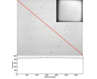
Figure 6. Uniform fluorescent glass imaged with a CELESTA Light Engine (Lumencor, Inc., Beaverton, OR) coupled by an 800 µm diameter optical fiber to a critical epi-illuminator installed in a Nikon Ti/Ti2 microscope. Image capture using Nikon 60X/1.4 NA Plan Apo objective and an Andor Zyla 5.5 (2560 x 2160 pixels) sCMOS camera. The plot shows the gray level values recorded by the camera along the diagonal axis marked in red. The inset in the upper right hand corner shows the same sample imaged with a Nikon 10X/0.3 NA Plan Apo objective.